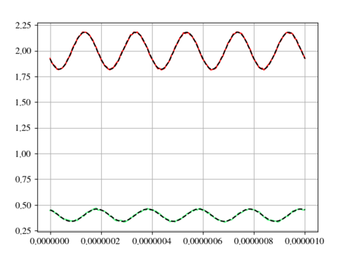
我很想知道兩種正弦波類型之間的相移。為此，我試圖用 scipy.cuve_fit 來擬合每一波。我一直在關注這個帖子。但是，我獲得了負幅度，并且相移有時看起來像轉發的 pi 弧度。我正在使用的代碼是下面的代碼：def fit_sin_LD(t_LD, y_LD):'''Fit sin to the input time sequence, and return fitting parameters "amp", "omega", "phase", "offset", "freq", "period" and "fitfunc"'''ff = np.fft.fftfreq(len(t_LD), (t_LD[1]-t_LD[0]))   # assume uniform spacingFyy = abs(np.fft.fft(y_LD))guess_freq = abs(ff[np.argmax(Fyy[1:])+1])   # excluding the zero frequency "peak", which is related to offsetguess_amp = np.std(y_LD) * 2.**0.5guess_offset = np.mean(y_LD)guess = np.array([guess_amp, 2.*np.pi*guess_freq, 0., guess_offset])def sinfunc_LD(t_LD, A, w, p, c):    return A * np.sin(w*t_LD + p) + c#boundary=([0,-np.inf,-np.pi, 1.5],[0.8, +np.inf, np.pi, 2.5])popt, pcov = scipy.optimize.curve_fit(sinfunc_LD, t_LD, y_LD, p0=guess, maxfev=3000) # with maxfev= number I can increase the number of iterationsA, w, p, c = poptf          = w/(2.*np.pi)fitfunc_LD = lambda t_LD: A*np.sin(w*t_LD + p) + cfitted_LD  = fitfunc_LD(t_LD)dic_LD = {"amp_LD": A, "omega_LD": w, "phase_LD": p, "offset_LD": c, "freq_LD": f, "period_LD": 1./f, "fitfunc_LD": fitted_LD, "maxcov_LD": np.max(pcov), "rawres_LD": (guess, popt, pcov)}return dic_LDdef fit_sin_APD(t_APD, y_APD):''' Fit sin to the input time sequence, and return fitting parameters "amp", "omega", "phase", "offset", "freq", "period" and "fitfunc" '''ff = np.fft.fftfreq(len(t_APD), (t_APD[1]-t_APD[0]))   # assume uniform spacingFyy = abs(np.fft.fft(y_APD))guess_freq = abs(ff[np.argmax(Fyy[1:])+1])   # excluding the zero frequency "peak", which is related to offsetguess_amp = np.std(y_APD) * 2.**0.5guess_offset = np.mean(y_APD)guess = np.array([guess_amp, 2.*np.pi*guess_freq, 0., guess_offset])我不明白為什么curve_fit會返回負幅度（就物理學而言沒有意義）。我也嘗試將邊界條件設置為 **kwargs* ：bounds=([0.0, -np.inf,-np.pi, 0.0],[+np.inf, +np.inf,-np.pi, +np.inf])但它會產生更奇怪的結果。我添加了一張顯示這種差異的圖片：有誰如何通過相位和幅度來克服這個問題？